02: Fitting Power Spectrum Models

Introduction to the module, beginning with the model object.

# Import the model object
from specparam import SpectralModel

# Import a utility to download and load example data
from specparam.utils.download import load_example_data

# Download example data files needed for this example
freqs = load_example_data('freqs.npy', folder='data')
spectrum = load_example_data('spectrum.npy', folder='data')

Model Object

At the core of the module is the SpectralModel object, which holds relevant data and settings as attributes, and contains methods to run the algorithm to parameterize neural power spectra.

The organization and use of the model object is similar to scikit-learn:

• A model object is initialized, with relevant settings

• The model is used to fit the data

• Results can be extracted from the object

Calculating Power Spectra

The SpectralModel object fits models to power spectra. The module itself does not compute power spectra. Computing power spectra needs to be done prior to using the specparam module.

The model is broadly agnostic to exactly how power spectra are computed. Common methods, such as Welch’s method, can be used to compute the spectrum.

If you need a module in Python that has functionality for computing power spectra, try NeuroDSP.

Note that model objects require frequency and power values passed in as inputs to be in linear spacing. Passing in non-linear spaced data (such logged values) may produce erroneous results.

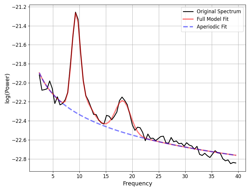
Fitting an Example Power Spectrum

The following example demonstrates fitting a power spectrum model to a single power spectrum.

# Initialize a model object
fm = SpectralModel()

# Set the frequency range to fit the model
freq_range = [2, 40]

# Report: fit the model, print the resulting parameters, and plot the reconstruction
fm.report(freqs, spectrum, freq_range)

WARNING: Lower-bound peak width limit is < or ~= the frequency resolution: 0.50 <= 0.49
        Lower bounds below frequency-resolution have no effect (effective lower bound is the frequency resolution).
        Too low a limit may lead to overfitting noise as small bandwidth peaks.
        We recommend a lower bound of approximately 2x the frequency resolution.

==================================================================================================

                                       POWER SPECTRUM MODEL

                        The model was run on the frequency range 2 - 40 Hz
                                 Frequency Resolution is 0.49 Hz

                            Aperiodic Parameters (offset, exponent):
                                         -21.6185, 0.7160

                                       3 peaks were found:
                                CF:   9.36, PW:  1.044, BW:  1.59
                                CF:  11.17, PW:  0.230, BW:  2.88
                                CF:  18.25, PW:  0.331, BW:  2.85

                                     Goodness of fit metrics:
                                    R^2 of model fit is 0.9829
                                    Error of the fit is 0.0356

==================================================================================================

Fitting Models with ‘Report’

The above method ‘report’, is a convenience method that calls a series of methods:

• fit(): fits the power spectrum model

• print_results(): prints out the results

• plot(): plots the data and model fit

Each of these methods can also be called individually.

# Alternatively, just fit the model with SpectralModel.fit() (without printing anything)
fm.fit(freqs, spectrum, freq_range)

# After fitting, plotting and parameter fitting can be called independently:
# fm.print_results()
# fm.plot()

WARNING: Lower-bound peak width limit is < or ~= the frequency resolution: 0.50 <= 0.49
        Lower bounds below frequency-resolution have no effect (effective lower bound is the frequency resolution).
        Too low a limit may lead to overfitting noise as small bandwidth peaks.
        We recommend a lower bound of approximately 2x the frequency resolution.

Model Parameters

Once the power spectrum model has been calculated, the model fit parameters are stored as object attributes that can be accessed after fitting.

Following scikit-learn conventions, attributes that are fit as a result of the model have a trailing underscore, for example:

• aperiodic_params_

• peak_params_

• error_

• r2_

• n_peaks_

Access model fit parameters from specparam object, after fitting:

# Aperiodic parameters
print('Aperiodic parameters: \n', fm.aperiodic_params_, '\n')

# Peak parameters
print('Peak parameters: \n', fm.peak_params_, '\n')

# Goodness of fit measures
print('Goodness of fit:')
print(' Error - ', fm.error_)
print(' R^2   - ', fm.r_squared_, '\n')

# Check how many peaks were fit
print('Number of fit peaks: \n', fm.n_peaks_)

Aperiodic parameters:
 [-21.61849464   0.71602468]

Peak parameters:
 [[ 9.36187745  1.04444653  1.58739815]
 [11.17320508  0.23009279  2.87553548]
 [18.24842747  0.33142173  2.84617078]]

Goodness of fit:
 Error -  0.03560699607369899
 R^2   -  0.9828918511262451

Number of fit peaks:
 3

Selecting Parameters

You can also select parameters using the get_params() method, which can be used to specify which parameters you want to extract.

# Extract a model parameter with `get_params`
err = fm.get_params('error')

# Extract parameters, indicating sub-selections of parameters
exp = fm.get_params('aperiodic_params', 'exponent')
cfs = fm.get_params('peak_params', 'CF')

# Print out a custom parameter report
template = ("With an error level of {error:1.2f}, an exponent "
            "of {exponent:1.2f} and peaks of {cfs:s} Hz were fit.")
print(template.format(error=err, exponent=exp,
                      cfs=' & '.join(map(str, [round(cf, 2) for cf in cfs]))))

With an error level of 0.04, an exponent of 0.72 and peaks of 9.36 & 11.17 & 18.25 Hz were fit.

For a full description of how you can access data with get_params(), check the method’s documentation.

As a reminder, you can access the documentation for a function using ‘?’ in a Jupyter notebook (ex: fm.get_params?), or more generally with the help function in general Python (ex: help(fm.get_params)).

Notes on Interpreting Peak Parameters

Peak parameters are labeled as:

• CF: center frequency of the extracted peak

• PW: power of the peak, over and above the aperiodic component

• BW: bandwidth of the extracted peak

Note that the peak parameters that are returned are not exactly the same as the parameters of the Gaussians used internally to fit the peaks.

Specifically:

• CF is the exact same as mean parameter of the Gaussian

• PW is the height of the model fit above the aperiodic component [1], which is not necessarily the same as the Gaussian height

• BW is 2 * the standard deviation of the Gaussian [2]

[1] Since the Gaussians are fit together, if any Gaussians overlap, than the actual height of the fit at a given point can only be assessed when considering all Gaussians. To be better able to interpret heights for individual peaks, we re-define the peak height as above, and label it as ‘power’, as the units of the input data are expected to be units of power.

[2] Gaussian standard deviation is ‘1 sided’, where as the returned BW is ‘2 sided’.

The underlying gaussian parameters are also available from the model object, in the gaussian_params_ attribute.

# Compare the 'peak_params_' to the underlying gaussian parameters
print('  Peak Parameters \t Gaussian Parameters')
for peak, gauss in zip(fm.peak_params_, fm.gaussian_params_):
    print('{:5.2f} {:5.2f} {:5.2f} \t {:5.2f} {:5.2f} {:5.2f}'.format(*peak, *gauss))

  Peak Parameters        Gaussian Parameters
 9.36  1.04  1.59         9.36  0.98  0.79
11.17  0.23  2.88        11.17  0.17  1.44
18.25  0.33  2.85        18.25  0.33  1.42

FitResults

There is also a convenience method to return all model fit results: get_results().

This method returns all the model fit parameters, including the underlying Gaussian parameters, collected together into a FitResults object.

The FitResults object, which in Python terms is a named tuple, is a standard data object used to organize and collect parameter data.

# Grab each model fit result with `get_results` to gather all results together
#   Note that this returns a FitResults object
fres = fm.get_results()

# You can also unpack all fit parameters when using `get_results`
ap_params, peak_params, r_squared, fit_error, gauss_params = fm.get_results()

# Print out the FitResults
print(fres, '\n')

# from specparamResults, you can access the different results
print('Aperiodic Parameters: \n', fres.aperiodic_params)

# Check the R^2 and error of the model fit
print('R-squared: \n {:5.4f}'.format(fm.r_squared_))
print('Fit error: \n {:5.4f}'.format(fm.error_))

FitResults(aperiodic_params=array([-21.61849464,   0.71602468]), peak_params=array([[ 9.36187745,  1.04444653,  1.58739815],
       [11.17320508,  0.23009279,  2.87553548],
       [18.24842747,  0.33142173,  2.84617078]]), r_squared=0.9828918511262451, error=0.03560699607369899, gaussian_params=array([[ 9.36187745,  0.97915803,  0.79369908],
       [11.17320508,  0.16895001,  1.43776774],
       [18.24842747,  0.33414213,  1.42308539]]))

Aperiodic Parameters:
 [-21.61849464   0.71602468]
R-squared:
 0.9829
Fit error:
 0.0356

Conclusion

In this tutorial, we have explored the basics of the SpectralModel object, fitting power spectrum models, and extracting parameters.

In the next tutorial, we will explore how this algorithm actually works to fit the model.