Note
Go to the end to download the full example code.
04: Periodic Component Fitting
Choosing and using different modes for fitting the periodic component.
# Import the model object
from specparam import SpectralModel

# Import function to check available list of modes
from specparam.modes import check_modes

# Import a utility to download and load example data
from specparam.demo import load_example_data
Component Fit Modes
So far, we have initialized spectral fitting without explicitly specifying what model we want to fit the the data. By doing so, we have been using the default model definition.
However, we can also control which model forms we fit to the data, separately for the periodic and aperiodic components. This is done by explicitly specifying Fit Modes for each model component.
In this part of the tutorial, we will explore how this works for the periodic component.
Periodic Fitting Approaches
As we’ve already seen, to fit putatively periodic activity - operationalized as regions of power over above the aperiodic component - the model fits ‘peaks’.
However, in order to actually do this, we need to specify a mathematical definition of how to describe these peaks. Specifying this fit function is what is meant by choosing the periodic mode.
To see the available periodic fit modes, we can use the
check_modes() function.
# Check the list of periodic modes
check_modes('periodic')
==================================================================================================

                                     AVAILABLE PERIODIC MODES

                                            'gaussian'
                                   Gaussian peak fit function.
                                        'skewed_gaussian'
                                Skewed Gaussian peak fit function.
                                             'cauchy'
                                    Cauchy peak fit function.
                                             'gamma'
                                    Fit a gamma peak function.
                                            'triangle'
                                   Triangle peak fit function.

==================================================================================================
Gaussian Periodic Mode
We will start with choosing the Gaussian fit mode.
# Download example data files needed for this example
freqs = load_example_data('freqs.npy', folder='data')
spectrum = load_example_data('spectrum.npy', folder='data')
# Initialize a model object, explicitly specifying periodic fit to 'gaussian'
fm1 = SpectralModel(periodic_mode='gaussian')

# Check the defined fit modes of the model object
fm1.modes.print()
==================================================================================================

                                            FIT MODES

                                     Aperiodic Mode : 'fixed'

                                    Periodic Mode : 'gaussian'

==================================================================================================
# Fit the model and report results
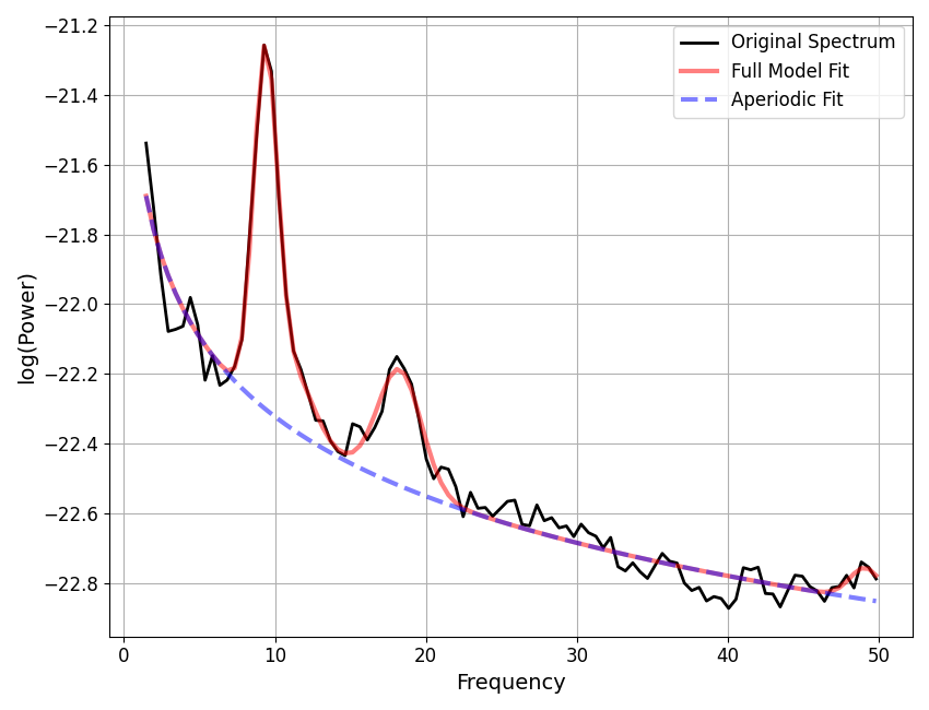
fm1.report(freqs, spectrum)

WARNING: Lower-bound peak width limit is < or ~= the frequency resolution: 0.50 <= 0.49
        Lower bounds below frequency-resolution have no effect (effective lower bound is the frequency resolution).
        Too low a limit may lead to over-fitting noise as small bandwidth peaks.
        We recommend a lower bound of approximately 2x the frequency resolution.

==================================================================================================

                                      SPECTRUM MODEL RESULTS

                       The model was fit with the 'spectral_fit' algorithm
               Model was fit to the 1-50 Hz frequency range with 0.49 Hz resolution

                               Aperiodic Parameters ('fixed' mode)
                                        (offset, exponent)
                                         -21.5643, 0.7580

                         Peak Parameters ('gaussian' mode) 4 peaks found
                                CF:   9.37, PW:   1.04, BW:   1.58
                                CF:  11.26, PW:   0.23, BW:   2.65
                                CF:  18.26, PW:   0.33, BW:   2.89
                                CF:  49.12, PW:   0.09, BW:   2.08

                                          Model metrics:
                                     error (mae) is 0.0366
                                  gof (rsquared) is 0.9831

==================================================================================================
Mathematical Description of the Periodic Component
You might notice that the above model looks the same as what we have fit previously. The Gaussian periodic mode is the default periodic mode.
Now that we have explicitly specified the Gaussian periodic fit mode, we can look into how the model is actually fit.
Each Gaussian, \(n\), referred to as \(G(F)_n\), is of the form:
This describes each peak in terms of parameters a, c and w, where:
\(a\) is the height of the peak, over and above the aperiodic component
\(c\) is the center frequency of the peak
\(w\) is the width of the peak
\(F\) is the array of frequency values
# Check the fit gaussian parameters
fm1.results.get_params('periodic', version='fit')
array([[ 9.36712113,  0.99082164,  0.78945133],
       [11.26311337,  0.16434593,  1.32426808],
       [18.25934079,  0.33386691,  1.44259835],
       [49.11921998,  0.09105003,  1.03933723]])
Fit vs. Converted Parameters
You might notice in the above, where we printed out the periodic parameters, that in doing so we specified explicitly to get the ‘fit’ version of the parameters, and that these parameters are actually a bit different than the peak parameters reported in the report above.
This is because the model manages two version of each component parameters: - fit: which reflect the original fit parameters, that define the model - converted: which reflect parameters after any relevant conversions
The reason we may want to apply to conversions to the parameters is that the fit versions, while defining the model, may not reflect what we actually want to analyze as outputs.
# Check the fit gaussian parameters
fm1.results.get_params('periodic', version='converted')
array([[ 9.36712113,  1.03782895,  1.57890265],
       [11.26311337,  0.22542876,  2.64853616],
       [18.25934079,  0.33089465,  2.8851967 ],
       [49.11921998,  0.08942602,  2.07867447]])
Converted Peak Parameters
The converted peak parameters are labeled as:
CF: center frequency of the extracted peak
PW: power of the peak, over and above the aperiodic component
BW: bandwidth of the extracted peak
The conversions that are applied to get these values are that:
CF is the exact same as mean parameter of the Gaussian
PW is the height of the model fit above the aperiodic component [1], which is not necessarily the same as the Gaussian height
BW is 2 * the standard deviation of the Gaussian [2]
[1] Since the Gaussians are fit together, if any Gaussians overlap, than the actual height of the fit at a given point can only be assessed when considering all Gaussians. To be better able to interpret heights for individual peaks, we re-define the peak height as above, and label it as ‘power’, as the units of the input data are expected to be units of power.
[2] Gaussian standard deviation is ‘1 sided’, where as the returned BW is ‘2 sided’.
Specifying a Different Fit Mode: Skewed Gaussian
As we saw above with check_modes there are also other periodic fit modes we can choose.
Next up, let’s try the skewed_gaussian mode.
# Initialize a model object, explicitly specifying periodic fit to 'gaussian'
fm2 = SpectralModel(periodic_mode='skewed_gaussian')

# Check the defined fit modes of the model object
fm2.modes.print()
==================================================================================================

                                            FIT MODES

                                     Aperiodic Mode : 'fixed'

                                Periodic Mode : 'skewed_gaussian'

==================================================================================================
# Fit the model and report results
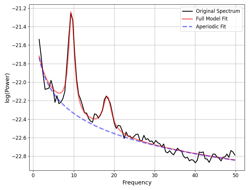
fm2.report(freqs, spectrum)
WARNING: Lower-bound peak width limit is < or ~= the frequency resolution: 0.50 <= 0.49
        Lower bounds below frequency-resolution have no effect (effective lower bound is the frequency resolution).
        Too low a limit may lead to over-fitting noise as small bandwidth peaks.
        We recommend a lower bound of approximately 2x the frequency resolution.

==================================================================================================

                                      SPECTRUM MODEL RESULTS

                       The model was fit with the 'spectral_fit' algorithm
               Model was fit to the 1-50 Hz frequency range with 0.49 Hz resolution

                               Aperiodic Parameters ('fixed' mode)
                                        (offset, exponent)
                                         -21.5643, 0.7580

                      Peak Parameters ('skewed_gaussian' mode) 4 peaks found
                         CF:   9.37, PW:   1.04, BW:   1.58, SKEW:  -0.00
                         CF:  11.31, PW:   0.23, BW:   2.65, SKEW:  -0.04
                         CF:  18.26, PW:   0.33, BW:   2.88, SKEW:   0.00
                         CF:  49.07, PW:   0.09, BW:   2.08, SKEW:   0.06

                                          Model metrics:
                                     error (mae) is 0.0366
                                  gof (rsquared) is 0.9831

==================================================================================================
In the above, we can see that the peaks are fit a bit differently.
Note that the resulting parameters are also different.
Specifying a Different Fit Mode: Cauchy
Finally, we can try the remaining periodic mode, the cauchy distribution!
# Initialize a model object, explicitly specifying periodic fit to 'gaussian'
fm3 = SpectralModel(periodic_mode='cauchy')

# Check the defined fit modes of the model object
fm3.modes.print()
==================================================================================================

                                            FIT MODES

                                     Aperiodic Mode : 'fixed'

                                     Periodic Mode : 'cauchy'

==================================================================================================
# Fit the model and report results
fm3.report(freqs, spectrum)
WARNING: Lower-bound peak width limit is < or ~= the frequency resolution: 0.50 <= 0.49
        Lower bounds below frequency-resolution have no effect (effective lower bound is the frequency resolution).
        Too low a limit may lead to over-fitting noise as small bandwidth peaks.
        We recommend a lower bound of approximately 2x the frequency resolution.

==================================================================================================

                                      SPECTRUM MODEL RESULTS

                       The model was fit with the 'spectral_fit' algorithm
               Model was fit to the 1-50 Hz frequency range with 0.49 Hz resolution

                               Aperiodic Parameters ('fixed' mode)
                                        (offset, exponent)
                                         -21.6133, 0.7244

                          Peak Parameters ('cauchy' mode) 2 peaks found
                                CF:   9.47, PW:   1.07, BW:   1.62
                                CF:  18.30, PW:   0.37, BW:   2.48

                                          Model metrics:
                                     error (mae) is 0.0431
                                  gof (rsquared) is 0.9772

==================================================================================================
That covers periodic mode selection!
Total running time of the script: (0 minutes 0.474 seconds)