Note
Go to the end to download the full example code.
05: Aperiodic Component Fitting
Choosing and using different modes for fitting the aperiodic component.
# Import the model object
from specparam import SpectralModel

# Import function to check available list of modes
from specparam.modes import check_modes

# Import a utility to download and load example data
from specparam.demo import load_example_data
Component Fit Modes
Just like for the periodic mode, the aperiodic component has different fit modes that can be applied to the data.
# Check the available aperiodic fit modes
check_modes('aperiodic')
==================================================================================================

                                    AVAILABLE APERIODIC MODES

                                             'fixed'
                                 One-over-f (powerlaw) function.
                                              'knee'
                    Lorentzian function, with a powerlaw exponent and a knee.
                                            'doublexp'
                     Multi-fractal powerlaw function (2 exponents & a knee).

==================================================================================================
Aperiodic Fit Mode: fixed
Fitting in the ‘fixed’ mode assumes a single 1/f like characteristic to the aperiodic component, meaning it looks linear across all frequencies in log-log space.
The ‘fixed’ aperiodic mode fits the aperiodic component with an offset and a exponent, using the following definition:
Note that this is the default aperiodic fit mode, and the one we have been using in the previous examples.
# Initialize a model object specifying a specific aperiodic fit mode
fm1 = SpectralModel(aperiodic_mode='fixed')

# Check the defined fit modes of the model object
fm1.modes.print()
==================================================================================================

                                            FIT MODES

                                     Aperiodic Mode : 'fixed'

                                    Periodic Mode : 'gaussian'

==================================================================================================
Relating Exponents to Power Spectrum Slope
The ‘fixed’ mode is equivalent to a linear fit in log-log space
Another way to measure 1/f properties in neural power spectra is to measure the slope of the spectrum in log-log spacing, fitting a linear equation as:
Where:
\(a\) is the power spectrum slope
\(b\) is the offset
\(F\) is the array of frequency values
In this formulation, the data is considered in log-log space, meaning the frequency values are also in log space. Since 1/f is a straight line in log-log spacing, this approach captures 1/f activity.
This is equivalent to the power spectrum model in this module, when fitting with no knee, with a direct relationship between the slope (\(a\)) and the exponent (\(\chi\)):
Aperiodic Fit Mode: knee
Another available aperiodic fit mode is the ‘knee’ mode, which includes a ‘knee’ parameter, reflecting a fit with a bend, in log-log space.
Adding a knee is done because also the although the assumption of a linear log-log property is typically true across some frequency ranges in neural data, it generally does not hold up across broad frequency ranges. If fitting is done in the ‘fixed’ mode, but the assumption of a single 1/f is violated, then fitting will go wrong.
Broad frequency ranges (typically ranges greater than ~40 Hz range) typically do not have a single 1/f, as assumed by ‘fixed’ mode, as they typically exhibit a ‘bend’ in the aperiodic component. This indicates that there is not a single 1/f property across all frequencies, but rather a ‘bend’ in the aperiodic component. For these cases, fitting should be done using an extra parameter to capture this, using the ‘knee’ mode.
# Initialize a new spectral model with the knee aperiodic mode
fm2 = SpectralModel(aperiodic_mode='knee')

# Check the defined fit modes of the model object
fm2.modes.print()
==================================================================================================

                                            FIT MODES

                                     Aperiodic Mode : 'knee'

                                    Periodic Mode : 'gaussian'

==================================================================================================
Mathematical Description of the Aperiodic Component
To fit the aperiodic component with a knee, we will use the following function \(L\):
Note that this function is fit on the semi-log power spectrum, meaning linear frequencies and \(log_{10}\) power values.
In this formulation, the parameters \(b\), \(k\), and \(\chi\) define the aperiodic component, as:
\(b\) is the broadband ‘offset’
\(k\) is the ‘knee’
\(\chi\) is the ‘exponent’ of the aperiodic fit
\(F\) is the array of frequency values
This function form is technically described as a Lorentzian function. We use the option of adding a knee parameter, since even though neural data is often discussed in terms of having 1/f activity, there is often not a single 1/f characteristic, especially across broader frequency ranges. Therefore, using this function form allows for modeling bends in the power spectrum of the aperiodic component, if and when they occur.
Note that if we were to want the equivalent function in linear power, using \(AP\) to indicate the aperiodic component in linear spacing, it would be:
Fitting with an Aperiodic ‘Knee’
Let’s explore fitting power spectrum models across a broader frequency range, using some local field potential data.
# Load example data files needed for this example
freqs = load_example_data('freqs_lfp.npy', folder='data')
spectrum = load_example_data('spectrum_lfp.npy', folder='data')
# Initialize a model object, setting the aperiodic mode to use a 'knee' fit
fm = SpectralModel(peak_width_limits=[2, 8], aperiodic_mode='knee')

# Check the defined fit modes of the model object
fm.modes.print()
==================================================================================================

                                            FIT MODES

                                     Aperiodic Mode : 'knee'

                                    Periodic Mode : 'gaussian'

==================================================================================================
# Fit a power spectrum model
#  Note that this time we're specifying an optional parameter to plot in log-log
fm.report(freqs, spectrum, [2, 70], plt_log=True)
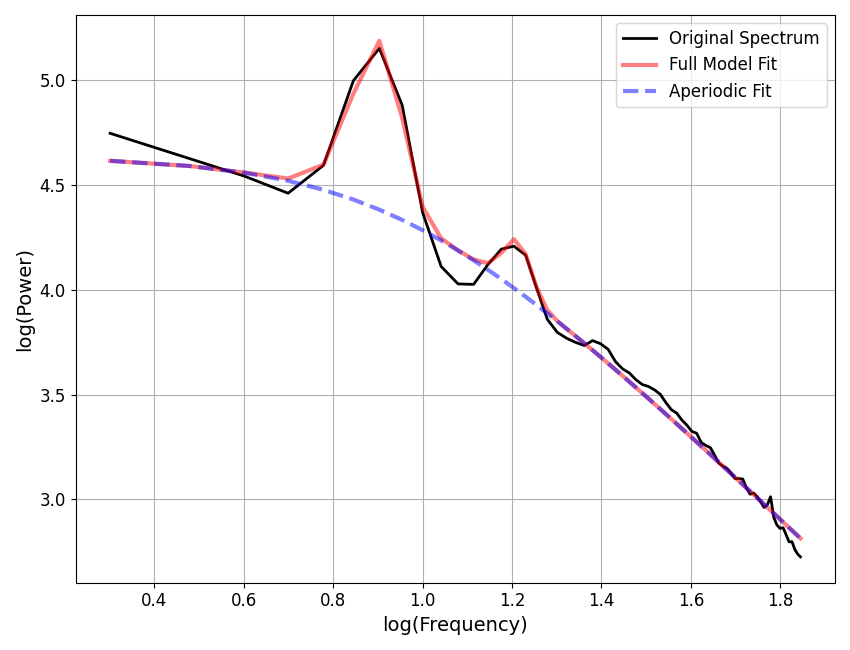
==================================================================================================

                                      SPECTRUM MODEL RESULTS

                       The model was fit with the 'spectral_fit' algorithm
               Model was fit to the 2-70 Hz frequency range with 1.00 Hz resolution

                                Aperiodic Parameters ('knee' mode)
                                     (offset, knee, exponent)
                                     6.5756, 87.1279, 2.0352

                         Peak Parameters ('gaussian' mode) 2 peaks found
                                CF:   7.98, PW:   0.81, BW:   2.03
                                CF:  16.32, PW:   0.23, BW:   2.30

                                          Model metrics:
                                     error (mae) is 0.0405
                                  gof (rsquared) is 0.9925

==================================================================================================
A note on interpreting the ‘knee’ parameter
The aperiodic fit has the form:
The knee parameter reported above corresponds to k in the equation.
This parameter is dependent on the frequency at which the aperiodic fit transitions from horizontal to negatively sloped.
To interpret this parameter as a frequency, take the \(\chi\)-th root of k, i.e.:
Interpreting the fit results when using knee fits is more complex, as the exponent result is no longer a simple measure of the aperiodic component as a whole, but instead reflects the aperiodic component past the ‘knee’ inflecting point. Because of this, when doing knee fits, knee & exponent values should be considered together.
Example: Aperiodic Fitting Gone Wrong
In the example above, we jumped directly to fitting with a knee.
Here we will explore what it looks like if we don’t use the appropriate mode for fitting the aperiodic component - fitting in ‘fixed’ mode when we should use ‘knee’
# Create and fit a power spectrum model in fixed mode to the same data as above
fm = SpectralModel(peak_width_limits=[2, 8], aperiodic_mode='fixed')
fm.report(freqs, spectrum, [2, 70], plt_log=True)
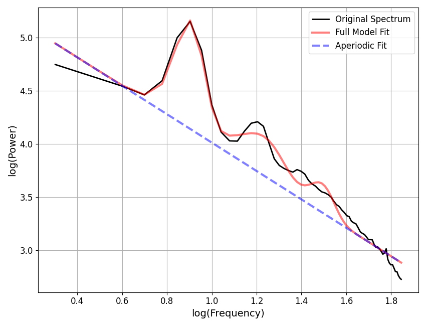
==================================================================================================

                                      SPECTRUM MODEL RESULTS

                       The model was fit with the 'spectral_fit' algorithm
               Model was fit to the 2-70 Hz frequency range with 1.00 Hz resolution

                               Aperiodic Parameters ('fixed' mode)
                                        (offset, exponent)
                                          5.3474, 1.3359

                         Peak Parameters ('gaussian' mode) 3 peaks found
                                CF:   8.01, PW:   1.02, BW:   2.41
                                CF:  17.02, PW:   0.37, BW:   8.00
                                CF:  31.02, PW:   0.27, BW:   8.00

                                          Model metrics:
                                     error (mae) is 0.0607
                                  gof (rsquared) is 0.9847

==================================================================================================
In this case, we see that the ‘fixed’ aperiodic component (equivalent to a line in log-log space) is not able to capture the data, which has a curve.
To compensate, the model adds extra peaks, but these are also not a good characterization of the data.
In this example, the data, over this frequency range, needs to be fit in ‘knee’ mode to be able to appropriately characterize the data.
Aperiodic Fit Mode: doublexp
Returning to our exploration of the available fit modes for the aperiodic component, another avaible fit mode is the ‘double exponent’ or ‘doublexp’.
In the above ‘knee’ mode, you might have noticed that even though the knee is described as a change in the value of the aperiodic exponent, implying there are two different exponent values, we still only fit one exponent value. In the above case, the exponent above the knee is fit, whereas the exponent below the knee is assumed to be zero.
By comparison, the double exponent model fits two different exponent values, above and below the knee.
# Create and fit a power spectrum model in doublexp aperiodic fit mode
fm = SpectralModel(peak_width_limits=[2, 8], aperiodic_mode='doublexp')
fm.report(freqs, spectrum, [2, 70], plt_log=True)
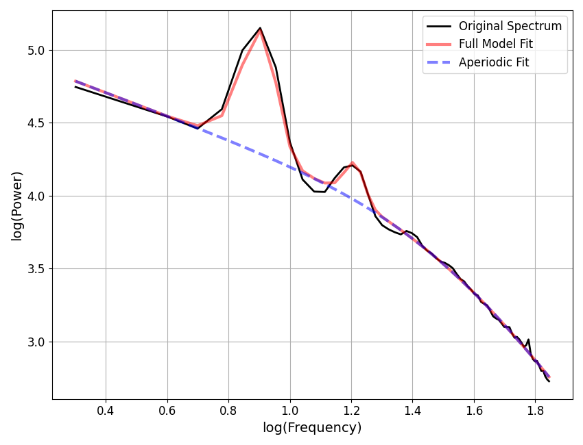
==================================================================================================

                                      SPECTRUM MODEL RESULTS

                       The model was fit with the 'spectral_fit' algorithm
               Model was fit to the 2-70 Hz frequency range with 1.00 Hz resolution

                              Aperiodic Parameters ('doublexp' mode)
                               (offset, exponent0, knee, exponent1)
                               5.6014, -133.4633, 6.1339, 134.9106

                         Peak Parameters ('gaussian' mode) 2 peaks found
                                CF:   7.98, PW:   0.85, BW:   2.13
                                CF:  16.27, PW:   0.25, BW:   2.41

                                          Model metrics:
                                     error (mae) is 0.0960
                                  gof (rsquared) is 0.9614

==================================================================================================
In the above example model fit, we can see that the aperiodic mode now includes 4 fit parameters, including two different exponent values (exponent1, reflecting below the knee, and exponent2, reflecting above the knee), as well as the offset and knee value.
Choosing an Aperiodic Fit Mode
It is important to choose the appropriate aperiodic fitting approach for your data.
If there is a clear knee in the power spectrum, fitting in ‘fixed’ mode will not work well. However fitting with a knee may perform sub-optimally in ambiguous cases (where the data may or may not have a knee), or if no knee is present.
Given this, we recommend:
Check your data, across the frequency range of interest, for what the aperiodic component looks like.
If it looks roughly linear (in log-log space), fit without a knee.
This is likely across smaller frequency ranges, such as 3-30.
Do not perform no-knee fits across a range in which this does not hold.
If there is a clear knee, then use a fit mode that includes a knee.
This is likely across larger fitting ranges such as 1-150 Hz.
Be wary of ambiguous ranges, where there may or may not be a knee.
Trying to fit without a knee, when there is not a single consistent aperiodic component, can lead to very bad fits. However, trying to fit with a knee may lead to suboptimal fits when no knee is present, and makes interpreting the exponent more difficult.
We therefore currently recommend picking frequency ranges in which the expected aperiodic component process is relatively clear.
Conclusion
We have now explored the SpectralModel object, and different fitting
approaches for the aperiodic component. Next up, we will be introducing how
to scale the fitting to apply across multiple power spectra.
Total running time of the script: (0 minutes 0.454 seconds)