Note
Go to the end to download the full example code.
06: Metrics & Model Evaluation
An overview of metrics & model evaluation to examine model fit quality.
# Import the model object
from specparam import SpectralModel

# Import function to check available list of metrics
from specparam.metrics import check_metrics

# Import a utility to download and load example data
from specparam.demo import load_example_data
Model Metrics
In this tutorial, we will explore model metrics.
The specparam module uses the term metric to refer to a measure that reflect something about the spectral model (but that is not computed as part of the model fit).
Generally, these metrics are used to evaluate how well the model fits the data and thus to assess the quality of the model fits.
The module comes with various available metrics. To see the list of available metrics,
we can use the check_metrics() function.
# Check the list of available metrics
check_metrics()
==================================================================================================

                                     AVAILABLE ERROR METRICS

                                            error_mae
                        Mean absolute error of the model fit to the data.
                                            error_mse
                         Mean squared error of the model fit to the data.
                                            error_rmse
                      Root mean squared error of the model fit to the data.
                                           error_medae
                       Median absolute error of the model fit to the data.

                                      AVAILABLE GOF METRICS

                                           gof_rsquared
                          R-squared between the model fit and the data.
                                         gof_adjrsquared
                      Adjusted R-squared between the model fit and the data.

==================================================================================================
As we can see above, metrics are organized into categories, including ‘error’ and ‘gof’ (goodness of fit). Within each category there are different specific measures.
Broadly, error measures compute an error measure reflecting the difference between the full model fit and the original data. Goodness-of-fit measures compute the correspondence between the model and data.
Specifying Metrics
Which metrics are computed depends on how the model object is initialized. When initializing a model object, which metrics to use can be specified using the metrics argument. When fitting a model, these metrics will then be automatically calculated after the model fitting and stored in the model object.
# Download example data files needed for this example
freqs = load_example_data('freqs.npy', folder='data')
spectrum = load_example_data('spectrum.npy', folder='data')
# Define a set of metrics to use
metrics1 = ['error_mae', 'gof_rsquared']

# Initialize model with metric specification
fm1 = SpectralModel(metrics=metrics1)

# Check the defined metrics from the model object
fm1.results.metrics.print()
==================================================================================================

                                         CURRENT METRICS

                                            error_mae
                                           gof_rsquared

==================================================================================================
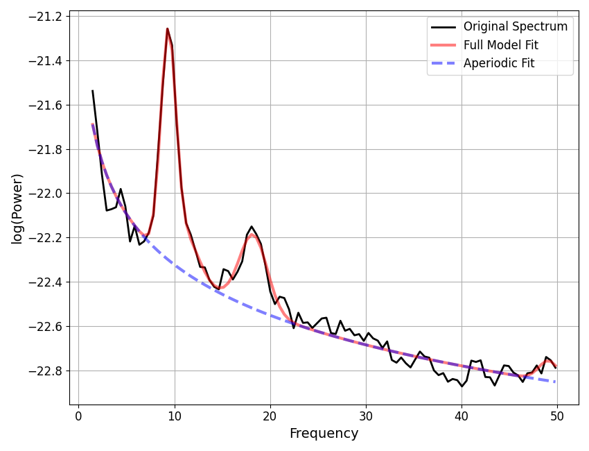
# Fit the model and report results
fm1.report(freqs, spectrum)
WARNING: Lower-bound peak width limit is < or ~= the frequency resolution: 0.50 <= 0.49
        Lower bounds below frequency-resolution have no effect (effective lower bound is the frequency resolution).
        Too low a limit may lead to over-fitting noise as small bandwidth peaks.
        We recommend a lower bound of approximately 2x the frequency resolution.

==================================================================================================

                                      SPECTRUM MODEL RESULTS

                       The model was fit with the 'spectral_fit' algorithm
               Model was fit to the 1-50 Hz frequency range with 0.49 Hz resolution

                               Aperiodic Parameters ('fixed' mode)
                                        (offset, exponent)
                                         -21.5643, 0.7580

                         Peak Parameters ('gaussian' mode) 4 peaks found
                                CF:   9.37, PW:   1.04, BW:   1.58
                                CF:  11.26, PW:   0.23, BW:   2.65
                                CF:  18.26, PW:   0.33, BW:   2.89
                                CF:  49.12, PW:   0.09, BW:   2.08

                                          Model metrics:
                                     error (mae) is 0.0366
                                  gof (rsquared) is 0.9831

==================================================================================================
After model fitting, values of the computed metrics can be accessed with the
get_metrics() method.
print('Error: ', fm1.get_metrics('error', 'mae'))
print('GOF: ', fm1.get_metrics('gof', 'squared'))
Error:  0.03662237211401322
GOF:  0.9830951375540399
All the metric results are stored with a Metrics sub-component of the model results, from which you can also directly access all the metric results.
# Check the full set of metric results
print(fm1.results.metrics.results)
{'error_mae': np.float64(0.03662237211401322), 'gof_rsquared': np.float64(0.9830951375540399)}
Default Metrics
You might notice that when specifying the metrics above, we specified metrics that have been available during model fitting previously, even when we did not explicitly specify them.
The two specified metrics above are actually the default metrics, which are selected if no explicit metrics definition is given, as we’ve seen in previous examples.
Changing Metrics
We can use explicit metric specification to select different metrics to compute, as in the next example.
# Define a new set of metrics to use
metrics2 = ['error_mse', 'gof_adjrsquared']

# Initialize model with metric specification
fm2 = SpectralModel(metrics=metrics2)

# Check the defined metrics from the model object
fm2.results.metrics.print()
==================================================================================================

                                         CURRENT METRICS

                                            error_mse
                                         gof_adjrsquared

==================================================================================================
# Fit the model and report results
fm2.report(freqs, spectrum)

WARNING: Lower-bound peak width limit is < or ~= the frequency resolution: 0.50 <= 0.49
        Lower bounds below frequency-resolution have no effect (effective lower bound is the frequency resolution).
        Too low a limit may lead to over-fitting noise as small bandwidth peaks.
        We recommend a lower bound of approximately 2x the frequency resolution.

==================================================================================================

                                      SPECTRUM MODEL RESULTS

                       The model was fit with the 'spectral_fit' algorithm
               Model was fit to the 1-50 Hz frequency range with 0.49 Hz resolution

                               Aperiodic Parameters ('fixed' mode)
                                        (offset, exponent)
                                         -21.5643, 0.7580

                         Peak Parameters ('gaussian' mode) 4 peaks found
                                CF:   9.37, PW:   1.04, BW:   1.58
                                CF:  11.26, PW:   0.23, BW:   2.65
                                CF:  18.26, PW:   0.33, BW:   2.89
                                CF:  49.12, PW:   0.09, BW:   2.08

                                          Model metrics:
                                     error (mse) is 0.0022
                               gof (adjrsquared) is 0.9803

==================================================================================================
Adding Additional Metrics
We are also not limited to a specific number of metrics. In the following example, we can specify a whole selection of different metrics.
# Define a new set of metrics to use
metrics3 = ['error_mae', 'error_mse', 'gof_rsquared', 'gof_adjrsquared']

# Initialize model with metric specification & fit model
fm3 = SpectralModel(metrics=metrics3)

# Check the defined metrics from the model object
fm3.results.metrics.print()
==================================================================================================

                                         CURRENT METRICS

                                            error_mae
                                            error_mse
                                           gof_rsquared
                                         gof_adjrsquared

==================================================================================================
# Fit the model and report results
fm3.report(freqs, spectrum)

WARNING: Lower-bound peak width limit is < or ~= the frequency resolution: 0.50 <= 0.49
        Lower bounds below frequency-resolution have no effect (effective lower bound is the frequency resolution).
        Too low a limit may lead to over-fitting noise as small bandwidth peaks.
        We recommend a lower bound of approximately 2x the frequency resolution.

==================================================================================================

                                      SPECTRUM MODEL RESULTS

                       The model was fit with the 'spectral_fit' algorithm
               Model was fit to the 1-50 Hz frequency range with 0.49 Hz resolution

                               Aperiodic Parameters ('fixed' mode)
                                        (offset, exponent)
                                         -21.5643, 0.7580

                         Peak Parameters ('gaussian' mode) 4 peaks found
                                CF:   9.37, PW:   1.04, BW:   1.58
                                CF:  11.26, PW:   0.23, BW:   2.65
                                CF:  18.26, PW:   0.33, BW:   2.89
                                CF:  49.12, PW:   0.09, BW:   2.08

                                          Model metrics:
                                     error (mae) is 0.0366
                                     error (mse) is 0.0022
                                  gof (rsquared) is 0.9831
                               gof (adjrsquared) is 0.9803

==================================================================================================
Note that when using get_metrics, you specify the category and measure names.
To return all available metrics within a specific category, leave the measure specification blank.
print(fm3.get_metrics('error'))
print(fm3.get_metrics('error', 'mse'))
[0.03662237 0.00221921]
0.0022192074947718615
As before you can also check the full set of metric results from the object results.
print(fm3.results.metrics.results)
{'error_mae': np.float64(0.03662237211401322), 'error_mse': np.float64(0.0022192074947718615), 'gof_rsquared': np.float64(0.9830951375540399), 'gof_adjrsquared': np.float64(0.9803108072688229)}
Interpreting Model Fit Quality Measures
These scores can be used to assess how the model is performing. However interpreting these measures requires a bit of nuance. Model fitting is NOT optimized to minimize fit error / maximize r-squared at all costs. To do so typically results in fitting a large number of peaks, in a way that overfits noise, and only artificially reduces error / maximizes r-squared.
The power spectrum model is therefore tuned to try and measure the aperiodic component and peaks in a parsimonious manner, and, fit the right model (meaning the right aperiodic component and the right number of peaks) rather than the model with the lowest error.
Given this, while high error / low r-squared may indicate a poor model fit, very low error / high r-squared may also indicate a power spectrum that is overfit, in particular in which the peak parameters from the model may reflect overfitting by fitting too many peaks.
We therefore recommend that, for a given dataset, initial explorations should involve checking both cases in which model fit error is particularly large, as well as when it is particularly low. These explorations can be used to pick settings that are suitable for running across a group. There are not universal settings that optimize this, and so it is left up to the user to choose settings appropriately to not under- or over-fit for a given modality / dataset / application.
Defining Custom Metrics
In this tutorial, we have explored specifying and using metrics by selecting from measures that are defined and available within the module. You can also define custom metrics if that is useful for your use case - see an example of this in the Examples.
Total running time of the script: (0 minutes 0.464 seconds)