06: Fitting Models over Time

Use extensions of the model object to fit power spectra across time.

# Import the time & event model objects
from specparam import SpectralTimeModel, SpectralTimeEventModel

# Import Bands object to manage oscillation band definitions
from specparam import Bands

# Import helper utilities for simulating and plotting spectrograms
from specparam.sim import sim_spectrogram
from specparam.plts.spectra import plot_spectrogram

Parameterizing Spectrograms

So far we have seen how to use spectral models to fit individual power spectra, as well as groups of power spectra. In this tutorial, we extent this to fitting groups of power spectra that are organized across time / events.

Specifically, here we cover the SpectralTimeModel and SpectralTimeEventModel objects.

Fitting Spectrograms

For the goal of fitting power spectra that are organized across adjacent time windows, we can consider that what we are really trying to do is to parameterize spectrograms.

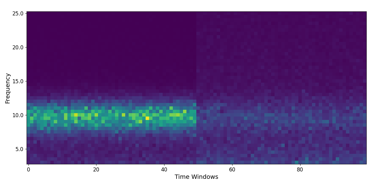
Let’s start by simulating an example spectrogram, that we can then parameterize.

# Create & plot an example spectrogram
n_pre_post = 50
freq_range = [3, 25]
ap_params = [[1, 1.5]] * n_pre_post + [[1, 1]] * n_pre_post
pe_params = [[10, 1.5, 2.5]] * n_pre_post + [[10, 0.5, 2.]] * n_pre_post
freqs, spectrogram = sim_spectrogram(n_pre_post * 2, freq_range, ap_params, pe_params, nlvs=0.1)

# Plot our simulated spectrogram
plot_spectrogram(freqs, spectrogram)

SpectralTimeModel

The SpectralTimeModel object is an extension of the SpectralModel objects to support parameterizing neural power spectra that are organized across time (spectrograms).

In practice, this object is very similar to the previously introduced spectral model objects, especially the Group model object. The time object is a mildly updated Group object.

The main differences with the SpectralTimeModel from previous model objects are that the data it accepts and parameterizes should be organized as as array of power spectra over time windows - basically as a spectrogram.

# Initialize a SpectralTimeModel model, which accepts all the same settings as SpectralModel
ft = SpectralTimeModel()

Defining Oscillation Bands

Before we start parameterizing power spectra we need to set up some guidance on how to organize the results - most notably the peaks. Within the object, the Time model does fit and store all the peaks it detects. However, without some definition of how to store and visualize the peaks, the object cannot visualize the results across time.

We can therefore use the Bands object to define oscillation bands of interest. By doing so, the Time model object will organize peaks based on these band definitions, so we can plot, for example, alpha peaks across time windows.

# Define a bands object to organize peak parameters
bands = Bands({'alpha' : [7, 14]})

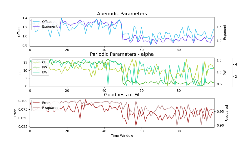
Now we are ready to fit our spectrogram! As with all model objects, we can fit the models with the fit method, or fit, plot, and print with the report method.

# Fit the spectrogram and print out report
ft.report(freqs, spectrogram, peak_org=bands)

Fitting model across 100 power spectra.

WARNING: Lower-bound peak width limit is < or ~= the frequency resolution: 0.50 <= 0.50
        Lower bounds below frequency-resolution have no effect (effective lower bound is the frequency resolution).
        Too low a limit may lead to overfitting noise as small bandwidth peaks.
        We recommend a lower bound of approximately 2x the frequency resolution.

==================================================================================================

                                           TIME RESULTS

                                 Number of time windows fit: 100

                        The model was run on the frequency range 3 - 25 Hz
                                 Frequency Resolution is 0.50 Hz

                              Power spectra were fit without a knee.

                                      Aperiodic Fit Values:
                        Exponents - Min:  0.849, Max:  1.804, Mean: 1.337

                          Periodic params (mean values across windows):
                      alpha - CF: 10.06, PW:  0.98, BW:  3.27, Presence: 1.0%

                          Goodness of fit (mean values across windows):
                            R2s -  Min:  0.897, Max:  0.992, Mean: 0.967
                         Errors -  Min:  0.026, Max:  0.103, Mean: 0.069

==================================================================================================

In the above, we can see that the Time object measures the same aperiodic and periodic parameters as before, now organized and plotted across time windows.

Parameterizing Repeated Events

In the above, we parameterized a single spectrogram reflecting power spectra over time windows.

We can also go one step further - parameterizing multiple spectrograms, with the same time definition, which can be thought of as representing events (for example, examining +/- 5 seconds around an event of interest, that happens multiple times.)

To start, let’s simulate multiple spectrograms, representing our different events.

# Simulate a collection of spectrograms (across events)
n_events = 3
spectrograms = []
for ind in range(n_events):
    freqs, cur_spect = sim_spectrogram(n_pre_post * 2, freq_range, ap_params, pe_params, nlvs=0.1)
    spectrograms.append(cur_spect)

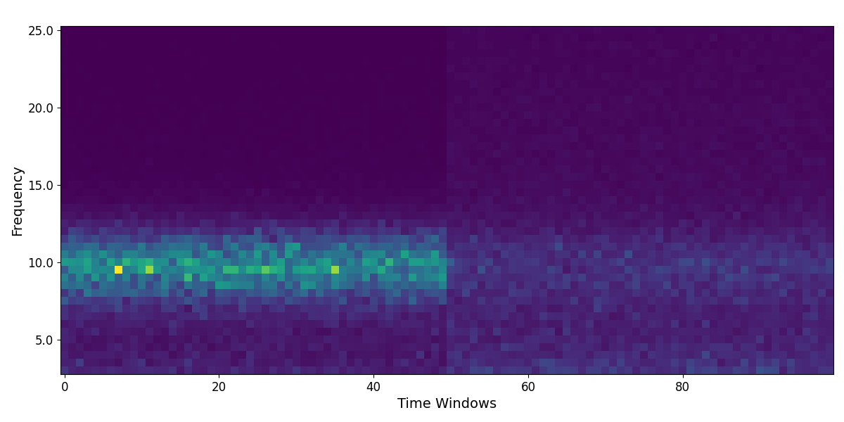
# Plot the set of simulated spectrograms
for cur_spect in spectrograms:
    plot_spectrogram(freqs, cur_spect)

• 
• 
• 

SpectralTimeEventModel

To parameterize events (multiple spectrograms) we can use the SpectralTimeEventModel object.

The Event is a further extension of the Time object, which can handle multiple spectrograms. You can think of it as an object that manages a Time object for each spectrogram, and then allows for collecting and examining the results across multiple events. Just like the Time object, the Event object can take in a band definition to organize the peak results.

The Event object has all the same attributes and methods as the previous model objects, with the notably update that it accepts as data to parameterize a 3d array of spectrograms.

# Initialize the spectral event model
fe = SpectralTimeEventModel()

# Fit the spectrograms and print out report
fe.report(freqs, spectrograms, peak_org=bands)

Fitting model across 3 events of 100 windows.
Fitting model across 100 power spectra.

WARNING: Lower-bound peak width limit is < or ~= the frequency resolution: 0.50 <= 0.50
        Lower bounds below frequency-resolution have no effect (effective lower bound is the frequency resolution).
        Too low a limit may lead to overfitting noise as small bandwidth peaks.
        We recommend a lower bound of approximately 2x the frequency resolution.

Fitting model across 100 power spectra.
Fitting model across 100 power spectra.
==================================================================================================

                                          EVENT RESULTS

                                     Number of events fit: 3

                        The model was run on the frequency range 3 - 25 Hz
                                 Frequency Resolution is 0.50 Hz

                              Power spectra were fit without a knee.

                             Aperiodic params (values across events):
                        Exponents - Min:  1.331, Max:  1.339, Mean: 1.335

                           Periodic params (mean values across events):
                     alpha - CF: 10.05, PW:  0.98, BW:  3.21, Presence: 100.0%

                             Goodness of fit (values across events):
                            R2s -  Min:  0.965, Max:  0.966, Mean: 0.966
                         Errors -  Min:  0.070, Max:  0.070, Mean: 0.070

==================================================================================================

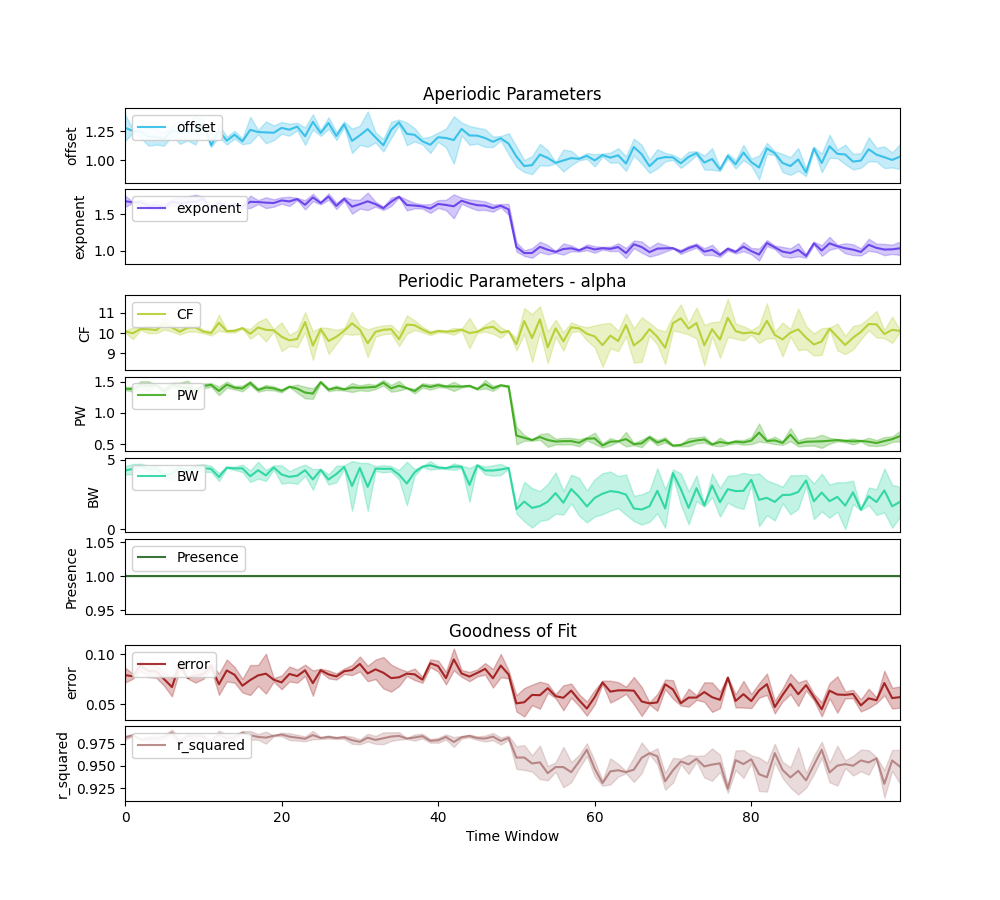
In the above, we can see that the Event object mimics the layout of the Time report, with the update that since the data are now averaged across multiple event, each plot now represents the average value of each parameter, shaded by it’s standard deviation.

When examining peaks across time and trials, there can also be a variable presence of if / when peaks of a particular band are detected. To quantify this, the Event report also includes the ‘presence’ plot, which reports on the % of events that have a detected peak for the given band definition. Note that only time windows with a detected peak contribute to the visualized data in the other periodic parameter plots.

Conclusion

Now we have explored fitting power spectrum models and running these fits across time windows, including across multiple events. Next we dig deeper into how to choose and tune the algorithm settings, and how to troubleshoot if any of the fitting seems to go wrong.