Note
Go to the end to download the full example code.
Custom Modes
This example covers defining and using custom fit modes.
# Import functionality used to define custom fit modes
from collections import OrderedDict
import numpy as np

# Import the model object
from specparam import SpectralModel

# Import function to simulate a power spectrum
from specparam.sim import sim_power_spectrum

# Import objects used to define a custom mode
from specparam.modes.mode import Mode
from specparam.modes.paramdef import ParamDefinition
Defining Custom Fit Modes
As covered in the tutorials, the specparam module has a set of predefined fit modes, wherein modes refer to the fit function and associated metadata & description that describes how each component is fit.
In this tutorial, we will explore how you can also define your own custom modes.
To do so, we will start by simulating an example power spectrum to use for this example.
# Define simulation parameters
ap_params = [0, 1]
gauss_params = [10, 0.5, 2, 20, 0.3, 2]
nlv = 0.0025

# Simulate an example power spectrum
freqs, powers = sim_power_spectrum(\
    [1, 40], {'fixed' : ap_params}, {'gaussian' : gauss_params}, nlv, freq_res=0.25)
Example: Custom Aperiodic Mode
To start, we will define a custom aperiodic fit mode. Specifically, we will define a custom aperiodic fit mode that fits only a single exponent.
In theory, such an aperiodic fit mode could be used if one knew that the offset for all power spectra of interest had an offset of 0 (for example, if they were all normalized as such), but in practice this is not likely to be a useful fit mode, and is used here merely as a simplified example of defining a custom fit mode. That is, while this is a functioning custom fit mode definition for the sake of an example, this is not necessarily a useful (or recommended) fit function.
First, we need to define a fit function that can be applied to fit our component.
To do so, we define a function that defines the fit function. To be able to be used in a model object, this function needs to follow a couple key principles:
the first input should be for x-axis values of the data to be modeled (frequencies)
regardless of how many parameters the fit function has, these should be organized as *args in the function definition
the body of function should unpack the params, fit the function definition to the input data, and then return the model result (modeled component)
By following these conventions, the model object is able to use this function to fit the specified component, passing in data and parameters appropriately, regardless of the set of parameters and function definition.
# Define a custom aperiodic fit function
def expo_only_function(xs, *params):
    """Exponent only aperiodic fit function

    Parameters
    ----------
    xs : 1d array
        X-axis values.
    *params : float
        Parameters that define the component fit: exponent.

    Returns
    -------
    ys : 1d array
        Output values of the fit.
    """

    exp = params
    ys = np.log10(xs**exp)

    return ys
Now that we have the fit function defined, we need to collect some additional information to be able to use our fit mode in the model object, starting with the parameter definition.
In order for the model object to have a description of the parameters that define the fit
mode, we use the ParamDefinition object.
To use this object, we use an OrderedDict to define a parameter description, where each key is a parameter name (this being the name that will be used to access the parameter from the model object), and a description of the parameter. Note that by using an OrderedDict, we ensure that the order of the parameters is consistent. Make sure the order of the parameters in the definition matches the order of the parameters in the fit function.
# Define the parameter definition for the expo only fit mode
expo_only_params = ParamDefinition(OrderedDict({
    'expo' : 'Exponent of the aperiodic component.',
}))
Now we have the main elements of our new fit mode, we can use the
Mode object to define the full mode. To do so, we initialize
a Mode object passing in metadata about the fit mode, as well our our fit function and
parameter definition.
Note that there is some meta-data that needs to be defined in the Mode definition, including:
name, component, description: describes the fit mode
jacobian: a function that computes the Jacobian for the fit function, which in some cases can speed up fitting.
ndim: the dimensionality of the output parameters, which should typically be 1 for aperiodic modes (returns a 1d array of parameters per model fit) and 2d for peak parameters (returns a 2d array of parameters across potentially multiple detected peaks)
freqs_space, powers_space : the expected spacing of the data
# Define the custom exponent only fit mode
expo_only_mode = Mode(
    name='custom_expo_only',
    component='aperiodic',
    description='Fit an exponent only.',
    formula=r'A(F) = 1/f^x',
    func=expo_only_function,
    jacobian=None,
    params=expo_only_params,
    ndim=1,
    freq_space='linear',
    powers_space='log10',
)
Our custom fit mode is now defined!
The use this fit mode, we can initialize a model object and pass in the custom fit mode to use for fitting.
Note that in this example, we will use SpectralModel for our example,
but you can also take the same approach to define custom fit modes with other model objects.
# Initialize model object, passing in custom aperiodic mode definition
fm = SpectralModel(aperiodic_mode=expo_only_mode)

# Check the defined modes of the object
fm.modes.print()
==================================================================================================

                                            FIT MODES

                               Aperiodic Mode : 'custom_expo_only'

                                    Periodic Mode : 'gaussian'

==================================================================================================
Now we can use the model object to fit some data.
# Fit model and report results
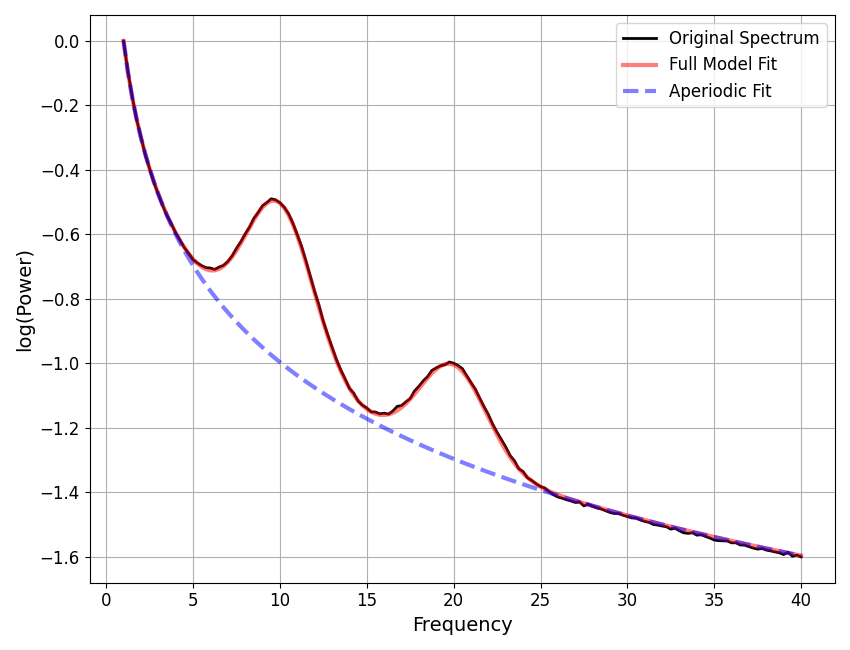
fm.report(freqs, powers)
==================================================================================================

                                      SPECTRUM MODEL RESULTS

                       The model was fit with the 'spectral_fit' algorithm
               Model was fit to the 1-40 Hz frequency range with 0.25 Hz resolution

                          Aperiodic Parameters ('custom_expo_only' mode)
                                              (expo)
                                             -0.9970

                         Peak Parameters ('gaussian' mode) 2 peaks found
                                CF:   9.99, PW:   0.49, BW:   3.94
                                CF:  19.99, PW:   0.29, BW:   3.87

                                          Model metrics:
                                     error (mae) is 0.0043
                                  gof (rsquared) is 0.9999

==================================================================================================
In the above report we can see that under the aperiodic mode section, the results reflect our custom fit mode!
Note that the parameter name is taken from what we described in the parameter definition. This is also the name you use to access the parameter results in get_params.
# Get the aperiodic parameters, using the custom fit mode parameter name
fm.get_params('aperiodic', 'expo')
np.float64(-0.9969963089207939)
Example Custom Periodic Fit Mode
Defining a custom fit mode can also be done in the same way for periodic modes.
In this example, we will define and apply a custom periodic fit mode that uses a rectangular peak fit function. Note that as we will see, this is not really a good peak option for neural data (though it may be useful for other data), but serves here as an example of
First, we start by defining a fit function, as before. This should follow the same format as introduced previously for the aperiodic fit mode function, with the added consideration that peak functions should be flexible for potentially having multiple possible peaks, meaning that the fit function needs to be set up in a way that multiple sets of parameters for multiple peaks can be passed in together, and the results summed together (e.g., if the fit function takes p parameters, the function should accept multiples of p number of inputs and loops across these, summing the resultant peaks).
# Define a custom peak fit function
def rectangular_function(xs, *params):
    """Custom periodic fit function - rectangular fit.

    Parameters
    ----------
    xs : 1d array
        X-axis values.
    *params : float
        Parameters that define the component fit: ctr, hgt, wid.

    Returns
    -------
    ys : 1d array
        Output values of the fit.
    """

    ys = np.zeros_like(xs)

    for ctr, hgt, wid in zip(*[iter(params)] * 3):
        ys[np.abs(xs - ctr) <= wid] += 1 * hgt

    return ys
Next up, as before, we need to define a parameter definition. Here, we will use the same labels as the standard (Gaussian) peak mode, redefined for the rectangle case.
# Define the parameter definition for a new periodic fit mode
rectangular_params = ParamDefinition(OrderedDict({
    'cf' : 'Center frequency of the rectangle.',
    'pw' : 'Power of the rectangle, over and above the aperiodic component.',
    'bw' : 'Width of the rectangle.'
}))
Finally, as before, we collect together all the required information to define our fit mode.
# Define the custom rectangular fit mode
rectangular_mode = Mode(
    name='rectangular',
    component='periodic',
    description='Custom rectangular (boxcar) peak fit function.',
    formula=None,
    func=rectangular_function,
    jacobian=None,
    params=rectangular_params,
    ndim=2,
    freq_space='linear',
    powers_space='log10',
)
Now we can initialize a model object with our custom periodic fit mode, and use it to fit some data!
# Initialize model object, passing in custom periodic mode definition
fm = SpectralModel(periodic_mode=rectangular_mode, max_n_peaks=2)

# Check the defined modes of the object
fm.modes.print()
==================================================================================================

                                            FIT MODES

                                     Aperiodic Mode : 'fixed'

                                  Periodic Mode : 'rectangular'

==================================================================================================
# Fit model and report results
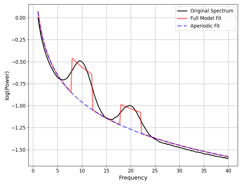
fm.report(freqs, powers)
==================================================================================================

                                      SPECTRUM MODEL RESULTS

                       The model was fit with the 'spectral_fit' algorithm
               Model was fit to the 1-40 Hz frequency range with 0.25 Hz resolution

                               Aperiodic Parameters ('fixed' mode)
                                        (offset, exponent)
                                          0.0685, 1.0290

                        Peak Parameters ('rectangular' mode) 2 peaks found
                                CF:  10.00, PW:   0.40, BW:   4.25
                                CF:  20.00, PW:   0.24, BW:   4.25

                                          Model metrics:
                                     error (mae) is 0.0439
                                  gof (rsquared) is 0.9782

==================================================================================================
In the above, we can see the results of using the custom periodic mode peak fit function.
Relationship Between Fit Modes & Fit Algorithms
In these examples, we defined simple fit modes wherein the new functions are similar enough to the existing cases that they can be dropped in and still work with the default fit algorithm. There are some new fit modes that might not work well with the existing / default algorithm - for example, the default algorithm makes some assumptions about the peak fit function. This means that major changes to the fit modes may need to be defined in tandem with updates to the fitting algorithm to make it all work together. Relatedly, you might notice from the above mode definition that there are additional details that can be customized, such as the expected spacing of the data, that would also require coordination with making sure the fit algorithm is consistent with the defined fit modes.
Combining Custom Modes
As a final example, note that you can also combine custom periodic and aperiodic fit modes together.
# Initialize model object, passing in custom aperiodic & periodic mode definitions
fm = SpectralModel(aperiodic_mode=expo_only_mode, periodic_mode=rectangular_mode, max_n_peaks=2)

# Check the defined modes of the object
fm.modes.print()
==================================================================================================

                                            FIT MODES

                               Aperiodic Mode : 'custom_expo_only'

                                  Periodic Mode : 'rectangular'

==================================================================================================
# Fit model and report results
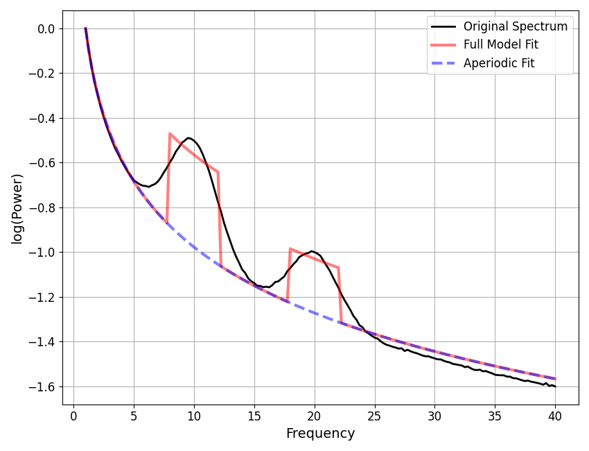
fm.report(freqs, powers)
==================================================================================================

                                      SPECTRUM MODEL RESULTS

                       The model was fit with the 'spectral_fit' algorithm
               Model was fit to the 1-40 Hz frequency range with 0.25 Hz resolution

                          Aperiodic Parameters ('custom_expo_only' mode)
                                              (expo)
                                             -0.9782

                        Peak Parameters ('rectangular' mode) 2 peaks found
                                CF:  10.00, PW:   0.41, BW:   4.25
                                CF:  20.00, PW:   0.24, BW:   4.25

                                          Model metrics:
                                     error (mae) is 0.0451
                                  gof (rsquared) is 0.9766

==================================================================================================
Adding New Modes to the Module
As a final note, if you look into the set of ‘built-in’ modes that are available within the module, you will see that these are defined in the exact way as done here - the only difference is that they are defined within the module and therefore can be accessed via their name, as a shortcut, rather than the user having to pass in their own full definitions.
This also means that if you have a custom mode that you think would be of interest to other specparam users, once the Mode object is defined it is quite easy to add this to the module as a new default option. If you would be interested in suggesting a mode be added to the module, feel free to open an issue and/or pull request.
Total running time of the script: (0 minutes 0.629 seconds)