Model Sub-Objects

Introducing the objects used within the model object.

In order to flexible fit model definitions to data, the Model object needs to manage multiple pieces of information, including relating to the data, the fit modes, the fit algorithm, and the model results. To do so, the model object contains multiple sub-objects, which each manage one of these elements.

The model object also have several convenience methods attached directly the object (e.g., fit, report, plot, get_params, etc) so that for most basic usage you don’t need to know the exact organization of the information within the model object. However, for more advanced analyses, and/or to start customizing model fitting, you need to know a bit about this structure. This example overviews the organization of the Model object, introducing each of the sub-objects.

# Define a helper function to explore object APIs
def print_public_api(obj):
    """Print out the public methods & attributes of an object."""
    print('\n'.join([el for el in dir(obj) if el[0] != '_']))

Data Object

The Data object manages data.

# Import the data object
from specparam.data.data import Data

# Import simulation function to make some example data
from specparam.sim import sim_power_spectrum

# Initialize a Data object
data = Data()

# Check the options available on the data object
print_public_api(data)

add_data
add_meta_data
checks
format
freq_range
freq_res
freqs
get_checks
get_meta_data
has_data
n_freqs
plot
power_spectrum
print
set_checks

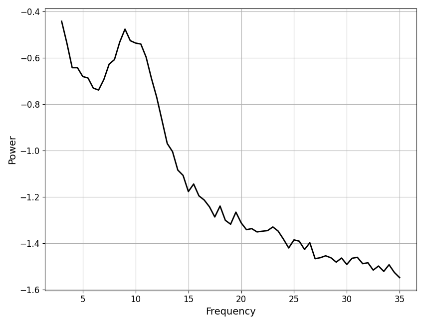
# Simulate an example power spectrum
freqs, powers = sim_power_spectrum([3, 35],
    {'fixed' : [0, 1]}, {'gaussian' : [10, 0.5, 2]}, nlv=0.025)

# Add data to data object
data.add_data(freqs, powers)

# Check some meta data from the data object
print('Frequency resolution:\t\t', data.freq_res)
print('Frequency range:\t\t', data.freq_range)

Frequency resolution:            0.5
Frequency range:                 [3.0, 35.0]

# Plot example data
data.plot()

# Check printed data summary
data.print()

==================================================================================================

                            The data object contains 1 power spectrum
                             with a frequency range of [3.0, 35.0] Hz
                              and a frequency resolution of 0.5 Hz.

==================================================================================================

Modes Object

The Modes object manages fit modes.

The Modes object itself contains individual mode definitions, which are implemented in Mode objects. Defining custom fit modes with the Mode object is covered in the custom modes example. Here we will import pre-defined mode definitions and explore the Modes object.

# Import the Mode & Modes objects, plus collections of pre-defined modes
from specparam.modes.modes import Modes
from specparam.modes.definitions import PE_MODES, AP_MODES

# Print out the available pre-defined modes
print(PE_MODES)
print(AP_MODES)

{'gaussian': MODE: periodic-gaussian, 'skewed_gaussian': MODE: periodic-skewed_gaussian, 'cauchy': MODE: periodic-cauchy}
{'fixed': MODE: aperiodic-fixed, 'knee': MODE: aperiodic-knee, 'doublexp': MODE: aperiodic-doublexp}

# Initialize a Modes object, passing in initialize Mode objects
modes = Modes(AP_MODES['fixed'], PE_MODES['gaussian'])

# Check the options available on the modes object
print_public_api(modes)

aperiodic
check_params
components
get_modes
get_params
periodic
print

# Print description of the modes
modes.print(True)

==================================================================================================

                                            FIT MODES

                                     Periodic Mode : gaussian
                     The approach taken for fitting the aperiodic component.
                                      Aperiodic Mode : fixed
                     The approach taken for fitting the aperiodic component.

==================================================================================================

Algorithm Object

The Algorithm object manages fit algorithms.

Defining custom fit algorithms with the Algorithm object is covered in the custom algorithms example. Here we will import pre-defined fit algorithms and explore the Algorithm object.

# Import the Algorithm object, plus collection of pre-defined algorithms
from specparam.algorithms.algorithm import Algorithm
from specparam.algorithms.definitions import ALGORITHMS

# Select and initialize an algorithm
algorithm = ALGORITHMS['spectral_fit']()

# Check the options available on the algorithm object
print_public_api(algorithm)

add_settings
data
data_format
description
get_debug
get_settings
modes
name
print
private_settings
public_settings
results
set_debug
settings

# Check the description of the algorithm
algorithm.description

'Original parameterizing neural power spectra algorithm.'

# Print out information about the algorithm
algorithm.print()

==================================================================================================

                                     ALGORITHM: spectral_fit

                                        ALGORITHM SETTINGS

                                 peak_width_limits : (0.5, 12.0)
                                        max_n_peaks : inf
                                      min_peak_height : 0.0
                                       peak_threshold : 2.0

==================================================================================================

Results Object

The Results object manages fit results.

# Import the Results object
from specparam.results.results import Results

# Initialize a results object
results = Results()

# Check the options available on the results object
print_public_api(results)

add_bands
add_metrics
add_results
bands
get_metrics
get_params
get_results
has_model
metrics
model
modes
n_params
n_peaks
params

Results Sub-Objects

As you may notice above, the Results object itself has several sub-objects to manage results information and related information.

This includes the Bands object, which manages frequency band definitions, and the Metrics object, which manages post-fitting evaluation metrics.

# Check the Bands object which is attached to the Results object
print(results.bands)

# Check the Metrics object which is attached to the Results object
print(results.metrics)

<specparam.metrics.metrics.Metrics object at 0x7f8ffa8351f0>

ModelParameters

The ModelParameters object manages model fit parameters.

# Import the ModelParameters object
from specparam.results.params import ModelParameters

# Initialize model parameters object
params = ModelParameters()

# Check the API of the object
print_public_api(params)

aperiodic
asdict
periodic
reset

# Check what object stores by exporting as a dictionary
params.asdict()

{'aperiodic_fit': nan, 'aperiodic_converted': nan, 'peak_fit': nan, 'peak_converted': nan}

ModelComponents

The ModelComponents object manages model components.

# Import the ModelComponents object
from specparam.results.components import ModelComponents

# Initialize model components object
components = ModelComponents()

# Check the API of the object
print_public_api(components)

get_component
modeled_spectrum
reset

Base Model Object

In the above, we have introduced the sub-objects that provide for the functionality of model fitting, including managing the data, fit modes, fit algorithm, and results.

Before the user-facing model objects, there is one final piece: the BaseModel object. This base level model object is inherited by all the model objects, providing a shared common definition of some base functionality.

# Import the base model object
from specparam.models.base import BaseModel

# Initialize a base model, passing in empty mode definitions
base = BaseModel(None, None, None, False)

# Check the API of the object
print_public_api(base)

add_modes
copy
get_data
modes
print_report_issue
print_settings
verbose

In the above, we can see that the BaseModel object implements a few elements that are common across all derived model objects, including includes the modes definition and a couple methods.

Model Objects

Finally, we get to the user-facing model objects!

Here, we will start with the SpectralModel object, initializing it as typically done as a user, and then explore the sub-objects.

To see more detail on how the Model object initializes and gets built based on all the sub-objects, see the implementation, including the __init__.

# Import a spectral model object
from specparam import SpectralModel

# Initialize a model object
fm = SpectralModel()

# Check the API of the object
print_public_api(fm)

add_data
add_modes
algorithm
copy
data
fit
get_data
get_metrics
get_params
load
modes
plot
print_report_issue
print_results
print_settings
report
results
save
save_report
to_df
verbose

# Check the sub-objects
print(type(fm.data))
print(type(fm.modes))
print(type(fm.algorithm))
print(type(fm.results))

<class 'specparam.data.data.Data'>
<class 'specparam.modes.modes.Modes'>
<class 'specparam.algorithms.spectral_fit.SpectralFitAlgorithm'>
<class 'specparam.results.results.Results'>

Looking into these sub-objects, you see that they are all the same as we introduced by initializing all these sub-objects one-by-one above, the only different being that they are now all connected together in the model object!

Derived model objects

Above, we used the SpectralModel object as an example object to introduce the structure of the model object & sub-objects.

The same approach is used for derived model objects (e.g. SpectralGroupModel) is used, the only difference being that as the shape and size of the data and results change, different versions of the data and results sub-objects are used (e.g. Data2D and Results2D).

# Import a spectral model object
from specparam import SpectralGroupModel, SpectralTimeModel, SpectralTimeEventModel

# Initialize a group model object
fg = SpectralGroupModel()

# Check the sub-objects
print(type(fg.data))
print(type(fg.results))

<class 'specparam.data.data.Data2D'>
<class 'specparam.results.results.Results2D'>

# Initialize a time model object
ft = SpectralTimeModel()

# Check the sub-objects
print(type(ft.data))
print(type(ft.results))

<class 'specparam.data.data.Data2DT'>
<class 'specparam.results.results.Results2DT'>

# Initialize an event model object
fe = SpectralTimeEventModel()

# Check the sub-objects
print(type(fe.data))
print(type(fe.results))

<class 'specparam.data.data.Data3D'>
<class 'specparam.results.results.Results3D'>